Data Structure
Introduction to Data Structure -:
Variables :-
->Variables
names are the placeholder for representing the data.
Data Types :-
->A
data type in a programming language is a set of data with the values having
predefined characteristics.
->System/Compiler
defined data type are called primitive data type.
->Structure
in c/c++
and classes in c++/java
are the means to create our own data type known as user defined data type.
Data Structure :-
->Data
structure is a particular way of storing and organizing data in a computer so
that it can be used efficiently.
Classification :-
->Two
major classification of data structure are :-
- Linear data structure (linked list, stack,
queue)
- Non linear data structure (tree, graph)
Abstract Data Type :-
->All
primitive data types supports basic operations like addition, subtraction, etc.
->The
system is providing the implementation for the primitive data type.
->For
non primitive data types , we also need to define operations.
->Combination
of data structure and their operations are known as abstract data type.
->So
data structure is all about creating abstract data type.
->Any
piece of information can be handled by defining appropriate data type and set
of possible operations.
Analysis of Algorithm -:
Algorithm :-
->An
algorithm is the step by step instruction to solve a given problem.
Eg :- sum()
= Algorithm to add first n natural numbers. Assume s is
a variable initialized to 0.
1) if
n<=0 return -1
2)
Repeat step 3 and 4 while n!=0
3) s
= s + n
4) [
decrement n ] n—
5)
returns
Analysis of Algorithm :-
->
The goal of analysis of algorithm is to compare algorithm mainly in terms of
running time but also in terms of running time but also in terms of other
factors ( like memory , effort etc. )
Rate of Growth :-
->
The rate at which the running time increases as a function of input is called
rate of growth.
f(n) = n4 + 2n2 + 100n + 500
f(n) = n4 for some n>n0
Time
= f(n)
intersection point
N
= number of inputs
Types of analysis :-
->
To analyse the given algorithm we need to know on what inputs the algorithm is
taking less time and on what inputs the algorithm is taking huge.
- worst case
- average case
- best case
Asymptotic Notations :-
->
For all the three cases we need to identify the upper and lower bounds.
->
Syntax of representation of bounds are
- Big – O notation
- Omega -
notation
- Theta -
notation
1)Big – O Notation :-


-> O(g(n)) = { f(n) : there exist positive
constants c and c0 such that 0<=f(n)<=c*g(n) for all n>=n0 }
->
The statement f(n) = O(g(n)) state only that g(n) is an upper bound on the
value of f(n) for all n , n>=n0
Eg
: f(n) = n2+3n+1
2(g(n)) = 2n2
n
= 1 :- f(1) = 1+3+1=5 , 2(g(n)) = 2
n
= 2 :- f(2) = 15 , 2(g(2)) = 8
n
= 3 :- f(3) = 19 , 2(g(3)) = 18
n
= 4 :- f(4) = 29 , 2(g(4)) = 32
O(n2) = O(g(n))
2) Omega Notation :-


->
omega(g(n)) = { f(n) : there exist positive constants c and c0 such that
0<=c*g(n)<=f(n) for all n>=n0 }
->
The statement f(n) = omega(g(n)) states only that g(n) is only a lower bound on
the value of f(n) all n , n>=n0
3)Theta Notation :-

->
theta(g(n)) = { f(n) : there exist positive constants c1 and c2 and n0 such
that 0<=c1*g(n)<=f(n)<=c2*g(n) for all n>n0 }
Arrays In Data Structure -:
Arrays :-
->
Arrays are the collection of a finite number of homogeneous data elements.
->
Elements of the array are referenced respectively by an index set consisting of
n consecutive numbers and are stored respectively in successive memory
locations.
Program
:-
main(){
int
a[5];
a[0] = 45;
a[1] = 56;
}
->
The number n of elements is called the length or size of the array.
->
The array elements can be accessed in a constant time by using the index of the
particular element.
->To
access an array element , address of an element is computed as an offset from
the base address of the array and one multiplication is needed to compute what
is supposed to be added to the base address to get the memory address of the
element.
-> int a[5];
a[3]
= 47;
100 +
sizeof(int)
* 3 = 106
OR
base
address + sizeof(data
type) * 3(any no) = any no.
-> First
the size of an element of that data type is calculated and then it is
multiplied with the index of the element to get the value to be added to the
base address.
-> This
process takes one multiplication and one addition . Since these two operations
take constant time, we can say the array access can be performed in constant
time.
Array Dimensions :-
1D Array :-
->
A list of data items that can be represented by one variable name using only
one subscript and such variable is called one dimensional array.
2D Array :-
->
A list of data items that can be conceptualize as rows and column which can be
represented using one name and two subscript.
Recursion & Backtracking In DS -:
Recursion :-
->Any
function which calls itself is called recursive.
->A
recursive method solves a problem by calling a copy of itself to work on a
smaller problem.
->It
is important to ensure that the recursion terminates.
->Each
time the function call itself with a slightly simpler version of the original
problem.
Why Recursion ?
->Recursive
code is generally shorter and easier to write than iterator code.
Recursion :-
->It
terminates when a base case is reached.
->Each
recursive call requires extra space on the stack frame(i.e. memory ).
->Solution
to some problems are easier to formulate recursively.
Example :-
main()
{
int
k;
k = fun(3);
printf(“%d”,k);
}
int
fun(int
a) {
int
s;
if(a == 1)
return(a);
s = a + fun(a-1);
return(s);
}
Application :-
1)
Fibonacci Series
2)
Factorial of a number
3)
Merge , Sort, Quick Sort,
4)
Binary Search
5)
Tree Traversal
6)
Graph Traversal (DFS,
BFS)
7)
Dynamic Programming
8) Divide and Conquer Algorithm
9)
Tower of Hanoi
10)
Backtracking Algorithm
Backtracking :-
->
Backtracking is the method of exhausted search using divide and conquer.
->
Sometimes the best algorithm for a problem is to try all possibilities.
->
This is always slow.
Recursion Problem :-
->
Next we will discuss the following problems :
- Tower of Hanoi.
- Factorial
- Fibonacci Series
- Greatest Common Division
- Printing all Permutation of given string.
- Generate all strings of n bits of binary
digits.
->
Define power function , which could handle negative powers.
->
Write a recursive function to print entered characters in reverse order.
->
Write a recursive function to convert decimal to binary.
Tower of Hanoi -:


->
The tower of Hanoi is mathematical puzzle.
->
The objective of the puzzle is to move the entire stack to another rod.
Rules :-
->
Only one disk may be moved at a time.
->
Each move consists of taking the upper disk from one of the rods and sliding it
onto another rod , on the top of other disk that may already be present on that
rod.
->
No disk may be placed on the top of smaller disk.
Logic :-
->
Move the top n-1 disks from source to auxiliary tower.
->
Move the nth disk from source to destination tower.
->
Move the n-1 disk from auxiliary tower to destination tower.
->
Transferring the top n-1 disks from source to auxiliary tower can again be
thought as a fresh problem and can be solved in the same manner.
Interesting fact about Tower of Hanoi :-
-The
tower of Hanoi puzzle was invented by the French Mathematician “Edouard
Lucas” in 1883.
->The
number of moves required to correctly move a tower of 64 disks is.
2^64
– 1 = 18,446,744,073,709,551,615.
->
At a rate of one move per second , that is 584,942,417,355 years.
Solution :-
void
TOH(int
n, char beg, char aux, char end)
{
if(n>=1)
{
TOH(n-1, beg, end, aux);
printf(“%c
to %c \n “, beg, end);
TOH(n-1, aux, beg, end);
}
}
Factorial with Recursion -:
Program :-
long
factorial(int
n)
{
if(n>0)
return(n * factorial(n-1));
else
return(1);
}
main()
{
printf(“Factorial
of 5 is %ld”,
factorial(5));
getch();
}
Fibonacci Series with Recursion -:
Fibonacci Series :-
1
1 2 3 5 8 13 21 34 55 89 143….
=>fib(6)
=
fib(5) + fib(4)
=
fib(4) + fib(3) + fib(3) + fib(2)
=
fib(3) + fib(2) + fib(2) + fib(1) + fib(2) + fib(1) + fib(1)
=
fib(2) + fib(1) + fib(1) + fib(1) + 1 + fib(1) + 1 + 1
=
fib(1) + 1 + 1 + 1 + 1 + 1 + 1 + 1
= 1 +
1 + 1 + 1 + 1 + 1 + 1 + 1
= 8
Program :-
int
fib(int
n)
{
if(n==1 || n==2)
return(1);
return(fib(n-1) + fib(n-2));
}
main()
{
int
I;
for(i=1;
i<=10;
i++)
printf(“%d”,
fib(i));
getch();
}
Greatest Common Divisor -:
What Is GCD ?
Eg
:- 4,6
4 =
4 2
1
6 =
6 3
2 1
GCD(4,6)
= 2
GCD(4,6)
= GCD(4,6%4)
=
GCD(4,2)
=
GCD(4%2, 2)
=
GCD(0,2)
= 2
By Euclid Theorem :-
GCD(a,b)
if(a>b)
GCD(a%b,b)
else
GCD(a,b%a)
Program :-
int
GCD(int
a, int
b)
{
if(a==b)
return(a);
if(a%b==0)
return(b);
if(b%a==0)
return(a);
if(a>b)
return(GCD(a%b,b));
else
return(GCD(a,b%a));
}
STACK -:


What Is STACK ?
->A
stack is a list of elements in which an element may be inserted or deleted only
at one end , called the top of the stack.
->Stack
is a specialized data storage structure (ADT)
->Stack
is a linear data structure.
Array & Stack :-
->Unlike
arrays , access of elements in a stack is restricted.
->It
has two main functions push and pop.
->Insertion
in a stack is done using push function and removal from a stack is done using
pop function.
Representation :-
->Stack
allows access to only the last element inserted hence, an item can be inserted
or removed from the stack from one end called the top of the stack.
->It
is therefore , also called Last-In-First-Out (LIFO) list.
Implementation :-
->Stack
can be implemented as
- Array
- Dynamic Array
- Linked List
Array Implementation :-
->Operation
:-
- PUSH
- POP
Algorithm PUSH :-
PUSH(stack,
top, mastk,
item)
->This
procedure pushes an item onto a satck.
1)[stack
already filled]
If top==mastk,
then
print
overflow and return
2)
Set top==top+1
3)
Set stack[top]=item
4)
return.
Algorithm POP :-
POP(stack,
top, item)
->This
procedure deletes the top element of stack and assigns it to the variable item.
1)[stack
has an item to be removed ?]
If top==-1 , then
print
underflow and return
2)Set
item=stack[top]
3)Set
top=top-1
4)return
Stack using Array :-
//
A structure to represent a stack
struct
stack {
int
top;
unsigned
capacity;
int
*array;
};
Polish Notation -:
Polish Notation :-
->The
method of writing operators of an expression either before their operands or
after them is called the polish notation.
Ways of Writing :-
1)
Infix Notation
2)
Prefix Notation
3)
Postfix Notation
1) Infix Notation :-
->When
the operators exist between two operands then the expression is called infix
notation.
->Example
:
A + B (Infix)
2) Postfix Notation :-
->
When the operators are written after their operands then the expression is
called the postfix notation.
->Example
:
A + B (Infix)
AB+ (Postfix)
3) Prefix Notation :-
->
When the operators are written before their operands then the expression is
called the prefix notation.
->
Example :
A + B (Infix)
+AB (Prefix)
Infix to Postfix -:
Algorithm :-
1)
Push ‘(’ onto the stack and add ‘)’ to the end of Q
2)
Scan Q from left to right and repeat steps 3 and 6 for each element of Q until
the stack is empty.
3) If
an operand is encountered add it to P .
4) If
a left parenthesis is encountered , push it onto stack.
5) If
an operator is encountered , then
- Repeatedly is encountered , then to P each
operator which has the same precedence than X
- Add X to stack.
6) If
a right parenthesis is encountered , then
- Repeatedly pop from the stack and add to P
each operator until a left parenthesis is encountered .
- Remove the left parenthesis.
7)
Exit.
Postfix to Infix -:
Algorithm :-
1)
[Add Sentinel] Add a right parenthesis ‘)’ at the end of P.
2)
[Loop] Scan P from left to right and repeat steps 3 and 4 for each element of P
until the sentinel ‘)’ is encountered .
3)
[Handling of operands] if an operand is encountered , put it on stack.
4)
[Handling of operators] If an operand X is encountered then.
- Remove the two top elements of stack , where
A is the top elements and B is the next to top elements.
- Evaluate BXA
- Place the result of (BXA) back to on stack .
[End
If structure]
[End
Loop of step 2]
5)
[Result] Set value equal to the top element on stack.
6)[Finished]
.
Queue -:


Revise ADT :-
->
ADT : Abstract Data Type
->
ADT describes storage structure and set of operations.
->
Queue is an ADT.
What Is Queue :-
->
In Queue , the order in which the data arrives is important.
->
Queue is a line of items waiting to be served in sequential order.
->
A Queue is an ordered list in which insertions are done at one end (rear) and
deletions are done at other end (front).
->
Working principle is first in first out (FIFO).
Queue ADT :-
->
Storage structure :
- Array/Dynamic Array/Linked List
->
Operations :
- Insertion
- Deletion
Array Implementation of Queue :-
Operations :-
-
createQueue()
- isEmptyQueue()
- isFullQueue()
- queueSize()
- enQueue()
- deQueue()
- deleteQueue()
Structure of Queue :-
struct
ArrayQueue()
{
int
front, rear;
int
capacity;
int
*arry;
};
Tree -:


What Is Tree :-
->
A tree is a hierarchical data structure.
->
A tree is defined as a finite set of one or more data items (node) such that
1) There is a special node called the root of
the tree.
2) The remaining nodes are partitioned into
n>=0 disjoint subset, each of which is itself a tree , and they are called
sub-trees.
Terminologies :-
1) Degree :-
->
The number of sub trees of a node is called its degree.
2) Leaf :-
->
A node with degree zero is called leaf.
3) Terminal Nodes :-
->
The leaf node are also called the terminal nodes.
4) Degree of tree :-
->
The degree of the tree is maximum degree of the nodes in the tree.
5) Ancestors :-
->
The ancestors of a node are all the nodes along the path from the root to that
node.
6) Descendants :-
->
The descendants of a node are all the node along the path from node to terminal
node.
7) Level Number :-
->
Each node is assigned a level number . The root node of the tree is assigned a
level number 0. Every other node assign a level number which is 1 more than the
level number of its parent.
8) Generation :-
->Nodes
with the same level number are said to belong to the same generation.
9) Height/Depth :-
->
The height or depth of a tree is the maximum of nodes in a branch.
10) Edge :-
->
A line drawn from a node N of T to a successor is called an edge.
11) Path :-
->
Sequence of consecutive edges is called path.
12)
Branch :-
->
Path ending in a leaf is called a branch.
Binary Tree -:


What Is Binary Tree :-
->
A binary tree T is called as a finite set of elements , called nodes, such that
:
1) T
is empty (called the null tree or empty tree) , or
2) T
contains a distinguished node R , called the root of T , and the remaining
nodes of T form an ordered pair of disjoint binary trees T1 and T2.
Complete Binary Tree :-


->
A complete binary tree is defined as a binary tree whose non leaf nodes have
non empty left and right sub tree and all leaves are at the same level.
Almost Complete Binary Tree :-


->
A complete binary tree is defined as a binary tree whose non leaf nodes have
non empty left and right sub tree and all leaves are either at the level or
second last level.
Strict Binary Tree :-


->
A binary tree is called a strictly binary tree if every non leaf node in the
binary tree has non empty left and right sub tree.
->
It means each node will have either 0 or 2 children.
Extended Binary Tree :-


->
An Extended binary tree is a tree that has been transformed into a full binary
tree. This transformation is achieved by inserting special ‘external’ nodes
such that every ‘internal node’ has exactly two children.
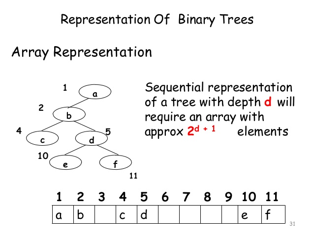
Representation of Binary Tree -:
There
are two possible representation of binary tree :-
1)
Array Representation
2)
Linked List Representation
Condition for
any representation :-
- One should
have direct access to the root R of T.
- Any node N
of T , one should have direct access to the children of N.

Linked Representation :-


->
Info is any information .
->
Left and Right are pointers to child nodes
Structure to represent a binary tree :-
struct
BinaryTreeNode
{
int
info;
struct
BinaryTreeNode
*left;
struct
BinaryTreeNode
*right;
};
Traversing of Binary Tree with
Recursion
-:
1) Pre-Order :-


->
Process the root R.
->
Traverse left sub tree of R in pre order.
->
Traverse the right sub tree of R in pre order.
2) In-Order :-


->
Traverse left sub tree of R in in order.
->
Process the root R.
->
Traverse the right sub tree of R in in order.
3) Post-Order :-


->
Traverse left sub tree of R in post order.
->
Traverse the right sub tree of R in post order.
->
Process the root R.
Pre order traversal :-
Recursive Approach :-
void
preOrder(struct
BinaryTreeNode
*root)
{ if(root)
{ print(“%d”,
root->info);
preOrder(root->left);
preOrder(root->right);
}
}
In order Traversal :-
Recursive Approach :-
void
inOrder(struct
BinaryTreeNode
*root)
{ if(root)
{ inOrder(root->left);
printf(“%d”,root->info);
inOrder(root->right);
}
}
Pre order Traversal :-
Recursive Approach :-
void
postOrder(struct
BinaryTreeNode
*root)
{ if(root)
{ postOrder(root->left);
postOrder(root->right);
printf(“%d”,
root->info);
}
}
Level Order Traversal of Binary Tree -:


->
Visit the root.
->
While traversing level L , keep all the elements at level L+1 in queue.
->
Go to the next level and visit all the nodes at the level.
->
Repeat
this until all levels are completed .
Void levelOrder(struct BinaryTreeNode *root)
{
struct BinaryTreeNode *temp;
struct Queue *Q = createQueue();
if(!root)
return;
enQueue(Q, root);
while(!isEmptyQueue(Q))
{
temp = deQueue(Q);
printf(“%d”,
temp->info);
if(temp->left)
enQueue(Q,
temp->left);
if(temp->right)
enQueue(Q,
temp->right);
}
deleteQueue(Q);
}
Binary Search Tree -:


->
In binary search tree , all the left sub tree elements should be less than root
data and all the right sub tree elements should be greater than root data .
This is called binary search tree.
->
This property should be satisfied at every node in the tree.
Structure to represent a BST :-
struct
BSTNode
{ int
data;
struct
BSTNode
*left;
struct
BSTNode
*right;
};
Elementary Operations :-
1)
Find
2)
Insertion
3)
Deletion
AVL Tree -:


Problem with BST :-
->
The disadvantage of a skewed binary search tree is that the worst case time
complexity of a search is O(n).
AVL :-
->
There is a need to maintain the binary search tree to be of balanced height ,
so that it is possible to obtained for the search option a time complexity of
O(log n) in the worst case .
->
One of the most popular balanced tree was introduced by Adelson
– Velskii
and Landis (AVL) .
-> An Empty binary tree is an AVL tree.
->
A non empty binary tree T is an AVL tree iff
given T^l
and t^r
to be the left and right sub tree of T and h(T^l)
and h(T^r)
to be the heights of sub trees T^l
and T^r
respectively , T^l
and T^r
are AVL trees and | h(T^l)
– h(T^r)
| <= 1
Searching In AVL Tree :-
->
Searching an AVL search tree for an element is exactly similar to the method
used in a binary search tree.
Insertion In AVL Tree :-
->
If after insertion of the element , the balance factor of any node in the tree
is affected so as to render the binary search tree unbalanced , we sort to
technique called rotations to restore the balance of the search tree.
Rotation In AVL Tree -:
->
To perform the rotations it is necessary to identify a specific node A whose
balance factor (BF) is neither 0, 1 or -1 and which is the nearest ancestor to
the inserted node on the path from the inserted node to the root.
Rotation Types :-
1) LL Rotation :-
->
Inserted node is in the left sub tree of left sub tree of node A.
2) RR
Rotation :-
->
Inserted node is in the right sub tree of right sub tree of node A.
3) LR
Rotation :-
->
Inserted node is in the right sub tree of left sub tree of node A.
4) RL
Rotation :-
->
Inserted node is in the left sub tree of right sub tree of node A.
What Is Heap -:


->
A heap is a tree with some special properties.
->
The basic requirement of a heap is that the value of a node must be >= (or
<=) to the values of its children.
->
The heap also has the additional property that all leaves should be at h or h-1
levels for some h>0
Types of Heap :-
1)
Min Heap
2)
Max Heap
Representation of Heap :-
->
Heap can be represented using arrays.
->
if index represent -> i
->
then child
left = 2 * i
+ 1
right = 2 * i
+ 2
->
for parent node index = (i
– 1)/2
Eg
:- (3-1)/2 = 1
(4-1)/2 = 1.5 = 1
Insertion and Deletion in a Heap :-
1)
Insertion In a Heap :-
2) Deletion In
Heap :-
Threaded Binary Tree -:
-> There
are two types of threaded binary trees
- Single
threaded
- Double
threaded
1) Single Threaded :-


->
Where a NULL right pointers is made to point to the in-order successor (if
successor exists).
2) Double Threaded :-


->
Where both left and right NULL pointers are made to point to in-order
predecessor and in-order successor respectively.
1) Single Threaded :-
2) Double Threaded :-
Threaded BT :-
->
In a simple threaded binary tree , the NULL right pointers are used to store
in-order successor.
->
Where ever a right pointers is NULL , it is used to store in-order successor.
Structure for Threaded BT :-
struct
Node
{ int
key;
struct
Node *left , *right;
bool isThreaded;
};
->
isThreaded
is used to indicate whether the right pointer is a normal right pointer or a
pointer to in-order successor.
Benefits of Threaded BT :-
->
The idea of threaded binary tree is to make in-order traversal faster and do it
without stack and without recursion.
M-Way Search Tree -:
M-Way Tree :-
-> A tree with maximum of m children is
known as M-Way tree.
M-Way Search Tree :-


->
M-Way search trees are generalized version of Binary search tree.
->
An M-Way search tree T may be an empty tree.
->
If T is non empty , it satisfies the following properties :
- Each node has , at most m child nodes
- If a node has k child nodes where k<=m ,
then the node can have only (k-1) keys k1 , k2 , ……k(k-1)
->
For a node A0 , (K1 , A1) , (K2 , A2) , ……..(k(m-1) , A(m-1)) all key values in
the sub tree pointed to by A , are less than the key K(i+1) , 0<=i<=m-2
, and all key values in the sub tree pointed to by A(m-1) are greater than
K(m-1).
->
Each of sub trees Aj
, 0<=i<=m-1
are also m-way search trees.
B Trees -:


->
B Tree is a special case of m-way search tree.
->
B Tree of order M satisfies the following properties :-
-
Each node has at most m children .
-
Each internal nodes has at least ceiling of m/2 children .
-
Root node has at least 2 children if it is not leaf.
- A
non leaf node with k children has k-1 keys.
- All
leaf nodes appear in the same level.
- For
root nodes -> (2,m)
-
internal nodes -> (ceil(m/2) , m)
-
Leaf nodes -> 0
Linear Search In Data Structure -:
-> Also
known as sequential search.
-> In this
search technique , we start at the beginning of a list or table and search for
the desired record by examining each subsequent record until either the desired
record is found or the list is exhausted.
Algorithm :-
->
Algorithm SEQSEARCH(L[] , N , ITEM) :- The algorithm find an ITEM in the list L
of N elements.
1)
[Initialize]
Set Flag = 1
2)
[Loop]
Repeat
step3 for k=0,1,2,3,4,……N-1
3)
If L[k] == ITEM then
a)
Set Flag = 0
b)
Write “Search Successful”
4)
If flag == 1 then : Write “Search Successful”
5)
[Finished]
Performance :-
->
Number of comparisons made in searching a record in a search table determine
the efficiency of the technique.
->
On an average the number of comparisons will be (n+1)/2.
->
The worst case efficiency of this algorithm is O(n).
Program :-
->
Write a function to implement linear search :-
void seq_search(int
L[], int
N, int
Item)
{ int
flag=1,k;
for(k=0; k<=N; k++)
{ if(L(k)
== Item)
{ flag=0;
printf(“Search
Successful”);
}
if(flag == 1)
printf(“Search
Successful”);
}
void main()
{ int
A[] = {22,44,11,77,88,55,99,33,66,1,100}
seq_search(A,11,66);
getch();
}
Binary Search -:
-> Search
for a particular item with a certain key resembles the search for a name in a
telephone directory.
-> The
approximate middle entry of the table is located and its key value is examined.
-> If its
value is too high , then the key value of the middle entry of the second half
of the table is examined and the procedure is repeated on the second half.
-> This
procedure is continued till the desired key is found or the search interval
become empty.
Algorithm :-
Algorithm
BINSEARCH(L[], N, Item) : The algorithm find an Item in the sorted list L of N
element .
1)
[Initialize]
Set l
= 0 , u = N -1
2)
[Loop]
Repeat step 3 and 4 while u>=l
3)
[get the mid point]
Set
m=(l+u)/2
4)
If Item = L[m] then :
write
“Successful Item Found”
Else if Item > L[m] then :
set
l=m+1
Else
set
u=m-1
[End
of loop]
5)
[Finished]
Hashing -:
Searching :-
->
We have seen various data structures like link list , arrays , trees etc.
->
Searching is a very frequent operation on any data structure.
Searching : Time Complexity :-
1)
Linked List :-
- O(n)
2)
Array (unsorted) :-
- O(n)
3)
Array (sorted) [Binary Search] :-
- O(log n)
4)
Binary Search Tree :-
- O(log n)
5)
Hash Table :-
- O(1)
Examples :-
1)To
store the key/value pair , we can use simple array like DS where keys directly
can be used as index to store values.
2)We
have 10 complaints indexed with a number ranges from 0 to 9 (say complaints
number).
3)We
have an array of 10 spaces to store 10 complaints.
4)Here
we can use complaints number as key and it is nothing but index number in an
array.
●
Hashing :-
In
case when keys are large and cannot be directly used as index to store values ,
we can use technique of hashing.
●
Hash Table :-
->
Mostly it is an array to store dataset .It is the data structure.
Hash Function :-
-
A hash function is any function that can be used to map dataset of arbitrary
size to dataset of fixed size which falls into the hash table.
- The
values returned a hash function are called hash values , hash codes , hash sums
, or simply hashes.
Hashing :-
-
In hashing large keys are converted into small ones by using hash functions and
then the values are stored in data structure called hash tables.
Hash Functions
- A hash
function usually means a function that compresses , meaning the output is
shorter than the input.
- A hash
function is any function that can be used to map data of arbitrary size to data
of fixed size.
Parameters of good Hash Function :-
-
Easy to compute.
-
Even Distribution.
-
Minimize Collisions.
Perfect Hashing :-
-
Perfect hashing maps each valid input to a different hash values (no
collision).
- A
good hash function to use with integer key values is the mid square method.
- The mid square method squares the key values
and then takes out the middle r bits of the result giving a value in the range
0 to 2^r - 1
Collision Resolution In Hashing
Recall Hashing :-
-
Hash table is a DS where the data elements are stored (inserted) , searched,
deleted based on the keys generated for each element , which is obtained from a
hashing function .
- A perfectly implemented hash table would
always promise an average insert / delete / retrieval time of O(1).
Collision :-
-
A situation when the resultant hashes for two or more data elements in the data
set , maps to the same location in the hash table , is called a hash collision
.
- In
such a situation two or more data elements would qualify to be stored / mapped
to the same location in the hash table.
Hash Collision Resolution :-
-
Two types of collision resolution
1) Open Hashing (Chaining)
2) Closed hashing (Open Addressing)
-
The difference between the two has to do with :-
- Whether collisions are stored outside the
table (open hashing ) or,
- Whether collisions result in storing one of
the records at another slot in the table (closed hashing).
Open Hashing :-
-
The simplest form of open hashing each slot in the hash table to be the head of
a linked list.
- All
records that hash to a particular slot are placed on that slots linked list.
Closed Hashing :-
a)
Linear Probing.
b)
Quadratic Probing.
c)
Double Hashing.
a)
Linear Proing
:-
b)
Quadratic Probing :-
c)Double
hashing :-
Bubble Sort
Sorting :-
-
Sorting is the process of arranging the data in some logical order.
-
This logical order may be ascending or descending in case of numeric values or
dictionary order in case of alphanumeric values.
- Two
types of Sorting :-
1) Internal Sorting.
2) External Sorting.
Bubble Sort :-
-
Bubble sort is very simple and easy to implement sorting technique . Until
unless explicitly stated sorting means ascending order.
Bubble Sort Logic :-
-
Lets take an example : we have a list of numbers stored an array.
-
Logic starts with comparison of first two elements and if the left element is
greater than right element , they swap their position . Comparison proceeds
till the end of array.
Algorithm :-
Bubble_sort(A,N)
: A is array of values and N is the number of elemets.
1)
Repeat for round = 1,2,3,…N-1
2) Repeat for i
= 0,1,2,…..N-1-round
3)
If A[i]
> A[i+1] then swap A[i]
and A[i+1]
4)
Return
Selection Sort
Working Logic :-
-Select the smallest value in the
first , swap smallest value with the first value of the list.
-Again Select the smallest value in
the list (exclude first value).
-Swap this value with the second
element of the list.
-Keep doing n-1 times to place all n
values in the sorted order.
Procedure MIN :-
-
Procedure MIN(A,K,N) : An array A is in memory . This procedure finds the
location LOC of the smallest element among A[K] , A[K+1] , ……A[N-1]
1)
[Initialize Pointers]
Set
MIN = A[K] and LOC = K;
2)
Repeat for j = K+1 , K+2, ……N-1;
If MIN>A[j] , then : Set MIN = A[j] and LOC
= j
[End of Loop]
3)
Return LOC
Algorithm :-
-
Algorithm SELECTION(A,N) : This algorithm sorts the array A with N elements.
1)
[Loop]
Repeat
steps 2 and 3 for K = 0,1,2,……..N-2;
2)
Call LOC = MIN=(A,K,N)
3)
[Interchange A[K] and A[LOC])
Set Temp = A[K] , A[K] = A[LOC]
A[LOC] = Temp
[End
of Loop]
4)
Exit
Insertion Sort
INS_Sort(A,N)
: A is an array with N elements
1) i=1;
2)
Repeat steps 3 to 5 while i<N
3)
temp = A[i]
, j = i-1
4)
Repeat while j>=0 and temp<A[j]
A[j+1] = A[j] and j = j-1
5)
A[j+1] = temp , I = i+1
6)
Exit.
Quick Sort
Quick Sort :-
-
Quick sort is an algorithm of the divide and conquer type . That is the problem
of sorting a set is reduced to the problem of sorting two smaller sets.
Procedure Quick :-
QUICK(A,N,BEG,END,LOC)
:- Here A is an array with N elements. Parameters BEG and END contain the
boundary values of the sub list of A to which this procedure applies. LOC keeps
track of the position of the first element.
1)
Set LEFT = BEG , RIGHT = END and LOC = BEG
2)
Scan from Right to Left
a) Repeat while A[LOC]<=A[RIGHT] and
LOC!=RIGHT;
RIGHT = RIGHT-1
b) If LOC == RIGHT than return
c) If A[LOC]>A[RIGHT] then swap A[LOC] and
A[LEFT]
also set LOC = LEFT and GoTo
step2
Algorithm QUICK_SORT :-
-
Algorithm QUICK SORT : This algorithm sorts an array A with N elements.
1)
TOP = -1
2) If
N>1 , then TOP = TOP +1 , LOWER[TOP]=0 , UPPER[TOP] = N-1;
3)
Repeat step 4 to 7 while TOP != -1
4)
POP Sub list from stack Set BEG = LOWER[TOP] ,
END = UPPER[TOP] , TOP
= TOP – 1
5)
Call QUICK(A,N,BEG,END,LOC)
6)
PUSH left sub list onto the stack
If(BEG < LOC-1) , then : TOP = TOP + 1,
LOWER[TOP] = BEG , UPPER[TOP] = LOC + 1
7)
PUSH right sub list onto stacks
If(LOC+1 < END) , then : TOP = TOP + 1,
LOWER[TOP] = LOC + 1, UPPER[TOP] = END
8)
Exit.
Heap Sort
Heap Sort :-
-
One main application of heap ADT is sorting , called Heap Sort.
LOGIC :-
-
Insert all elements of an unsorted array into the Heap.
-
Remove the maximum element (root node element) from the heap and exchange it
with the last value of array.
- Heapify.
-
Repeat the processes until heap remains with single element.
Algorithm :-
-
Algorithm HEAPSORT(A,N) : An array A with N elements is given . This algorithm
sorts the elements of A.
1)
[Build a heap H]
h = CreateHeap(N);
BuildHeap(h,A,N);
2)
Initialize
old_Size
= h->count;
3)
[Sort A by repeatedly deleting the root of H]
for(i=n;
i>0;
i--)
a) temp = h->array[0];
h->array[0] = h->array[h->count-1];
h->array[0] = temp;
b) h->count—
c) percolateDown(h,i)
4)
h->count = old_size;
5)
[Finished]
Merge Sort
Merge Sort :-
-
Merge Sort is an example of the divide and conquer approach.
- In
merge sort the unsorted list is divided into N sub lists each having one element.
Merge Sort Logic :-
-
A list of one element is considered sorted .
-
Then , it repeatedly merge these sub lists , to produce new sorted list is produced.
Algorithm :-
-
Let arr
be an array of N elements . Low is the lower bound and high is the upper bound
on arr.
1)
Declare variable mid
2)
Initialize low=0, high=N-1
3)
Calculate mid and divide the array into two sets.
if low!=high
mid= (low+high)/2
call Merge_Sort
recursively with
low = 0, high =mid
call Merge_Sort
recursively with
low = mid
+1, high
=N-1
call procedure
merging(Arr,low,mid,high)
[end of if]
4)Exit
Introduction to Graph
What Is Graph ?
-
A graph is an abstract data type that meant to implement the graph concepts
from mathematics.
- A
graph is a collection of nodes , connected by edges.
Data fit into Graph structure :-
-
Set of cities connected via rail route
- Set
of people , where some are friends.
-
Connection among computers (routers).
-
Tree is Graph.
Definition :-
1) In Computing :-
-
A graph is an abstract data structure that implements the mathematical
definition of a graph.
2) In Mathematics :-
-
A graph G is composed by a set of N vertices or nodes , connected through a set
of edges or links.
Definition of Graph :-
-
A graph G consists two things
1) A set V of elements called nodes or
vertices or points.
2) A set E of edges such that each edge e in E
is identified with a unique (unordered) pair of [u,v]
of nodes in V , denoted by e = [u,v].
- We
indicate the parts of the graph by writing G=(V,E).
Adjacent Nodes :-
-
If e = [u,v]
, then u and v are nodes called end points of e . U and v are said to be
adjacent nodes or neighbours.
Degree of Node :-
-
The degree of node u , written as deg(u)
, is the number of edges containing u.
Isolated Node :-
-
If deg(u)
= 0, then u is called an isolated node.
Closed Node :-
-
The path is said to be closed if Vo = Vn.
Vo V1 V2 V3 V4 Vo
or
Vo V1 V2 V4 V3 Vo
Connected Graph :-
-
A graph G is said to be connected if there is a path between any two of its
nodes.
Tree
-A connected graph T without any cycles is called a
tree graph or free tree or simply a tree.
-This means in particular , that there is a unique
simple path P between any two nodes u and v in T.
-If T is finite tree with m nodes then T will have m-1
edges.
Multiple edges :-
-
Distinct edges e and e` are called multiple edges if they connect the same and
points , that is if e=[u,v]
and e`=[u,v]
Loop :-
-
An edge is called a loop if it has identical end points , that is , if e=[u,v]
Multi-Graph :-
-
Multi graph is a graph consisting of multiple edges and loops.
Graph Types :-
1)
Directed Graph
2)
Undirected Graph
Directed Graph :-
-
A directed graph G also called diagraph or graph is same as multi-graph except
that each edge e in G is assigned a direction or in other words , each edge e
is identified with an ordered pair (u,v)
of nodes in G rather than an unordered pair [u,v].
-
Suppose G is directed graph with directed edges e=(u,v)
, Then e is also called an arc.
Complete Graph :-
-
A simple graph in which there exists an edge between every pair of vertices is
called a complete graph. It is also known as a universal graph or clique.
Null Graph :-
-
A graph without any edge is called a null graph.
- In
other words , every vertex in a null graph is an isolated vertex.
Sub-Graph :-
-
A graph G`=(V`,E`) is a sub graph of graph G=(V,E) if V` is a subset of V and
E` is a subset of E. Thus for G` to be a sub graph of graph G all the vertices
and edges of G` should be in G.
Representation of Graph
Graph DS :-
-
Graph is a set of nodes (vertices) and edges (lines connectivity vertices).
-
Real world information is sometimes a graph.
- To
represent real world information in a computer program , we need a DS called
graph data structure.
Graph ADT :-
-
Just like either ADT’s Graph ADT (data structure and set of operations) is used .
- To
create Graph ADT , we need to representation data structure in some way.
Representation of Graph DS :-
-
There are three ways to represent graph data structure.
1) Adjacency Matrix.
2) Adjacency List.
3) Adjacency Set.
Adjacency Matrix :-
-
To represent graph we need number of vertices , number of edges and also their
interconnections.
struct
Graph
{ int
V;
int
E;
int
**Adj;
};
Breadth First Search (BFS)
Graph Traversal :-
-
To solve problems on graphs , we need a mechanism for traversing the Graph.
-
Graph traversal algorithm are also known as graph search algorithm.
Graph Traversal Algorithm :-
1)
Breadth First Search (BFS)
2)
Depth First Search (DFS)
BFS :-
-
BFS uses queue.
-
Similar to level order traversing in tree.
Logic :-
-
During execution of algorithms , each node N of G will be in one of three status
of N.
- STATUS = 1 (Ready state)
- STATUS = 2 (Waiting state)
- STATUS = 3 (Processed state)
BFS Algorithm :-
-
Algorithm BFS :- This algorithm executes a breadth first search on a graph G
beginning at a starting node A.
1)
Initialize all nodes to the ready state (STATUS = 1).
2)
Put the
starting node A in QUEUE and change its status to the waiting state (STATUS = 2).
3)
[Loop] Repeat
steps 4 and 5 until QUEUE.
4)
Remove the front node N of QUEUE. Process
N and change the status of N to the
processed state (STATUS = 3).
5)
Add to the rear of QUEUE all the neighbours of N that are in the ready state
(STATUS = 1) and change their status to the waiting state (STATUS = 2)
[End
of step 3 Loop]
6)
Exit
Depth First Search
DFS :-
-
DFS uses Stack.
DFS Algorithm :-
-
Algorithm DFS : This algorithm executes a depth-first search on a graph G
beginning at a starting node A.
1)Initialize
all nodes to the ready state ( STATUS = 1)
2)Push
the starting node A onto Stack and change its status to the waiting state
(STATUS = 2).
3)[Loop]
Repeat steps 4 and 5 until Stack is empty.
4)Pop
the top node N of Stack . Process N and change its status to the processed
state (STATUS = 3).
5)Push
onto Stack all the neighbours of N that are still in the ready state (STATUS =
1) and change their status to the waiting state (STATUS = 2).
6)Exit.
Minimal Spanning Tree
1)Connect
2)Cost
Min
●
Minimal Spanning Tree :-
-We then wish to find an acyclic
subset T that connects all of the vertices and whose total weights is minimized
.
-Since , T is acyclic and connects
all of the vertices , it must form a tree , which we call a spanning tree since
it spans the graph G.
-We call the problem of determining
the tree T the minimum spanning tree problem.
Solution
:-
Two
algorithm for solving the minimum spanning tree problem .
-Kruskals
algorithm
-Prims Algorithm
Kruskal`s Algorithm
-It find a safe edge to add to the growing forest by
finding of all the edges that connect any two trees in the forest an edge [u,v] of least
weight.
Procedure :-
-Make – Set (v)
-Find – Set (u)
-Union (u,v)
Algorithm :-
1)[Initialize]
A:= Empty Set
2)[Loop]
for each vertex V belongs to V[G] do step 3
3)Make-Set(v)
4)Sort
the edges of E into non decreasing order by weight w.
5)[Loop]
for each edge [u,v]
belongs to E taken in non decreasing order by weight do step 6.
6)If
Find-Set(u) != Find-Set(v) then : A := A U {[u,v]}
, UNION(u,v).
7)Return
A.
Prim`s Algorithm
-Prim`s algorithm has the property
that the edges in the set A always form a single tree.
-The tree starts from an arbitrary
vertex r and grows until the tree spans all the vertices in V.
Procedure :-
-Extract-Min(Q)
Algorithm :-
-Algorithm MSTPRIM(G,w,r)
: All vertices that are not in the tree reside in a min property queue Q based
on a key field . For each vertex v , key[v] is the minimum weight of any edge
connecting v to a vertex in the tree ; by convention , key[v] = infinite . If
there is no such edge . The field pie(v) names the parent of v in the tree.
1)[Loop] for
each u belongs to v[G] step 2
2)Key[u] :=
infinite , pie(u) := NIL;
3)Key[r] :=0;
4)Q := v[G]
5)Repeat steps 6
to 8 while Q!=Empty set
6)U :=
EXTRACT-MIN(Q)
7)For each v
belongs to Q and Adj[u]
8)If v belongs
to Q and w(u,v)<key[v]
9)Then : pie[v]
:= u, key[v] := w(u,v)
10)Exit
Comments
Post a Comment